Error function

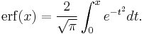
In mathematics, the error function (also called the Gauss error function) is a special function (non-elementary) of sigmoid shape which occurs in probability, statistics and partial differential equations. It is defined as:

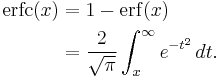
$\operatorname{erf}(x) = \frac{2}{\sqrt{\pi}}\int_{0}^x e^{-t^2} dt.$

The complementary error function, denoted erfc, is defined as

$\begin{align} \operatorname{erfc}(x) & = 1-\operatorname{erf}(x) \\ & = \frac{2}{\sqrt{\pi}} \int_x^{\infty} e^{-t^2}\,dt. \end{align}$

The imaginary error function, denoted erfi, is defined as

$\operatorname{erfi}(z) = -i\,\,\operatorname{erf}(i\,z)$

The complex error function, denoted w(x) and also known as the Faddeeva function, is defined as

$w(x) = e^{-x^2}{\operatorname{erfc}}(-ix) = e^{-x^2}[1%2Bi\,\,\operatorname{erfi}(x)]$

1 The name "error function"
2 Properties
3 Approximation with elementary functions
4 Applications
5 Related functions
- 5.1 Generalized error functions
- 5.2 Iterated integrals of the complementary error function
6 Implementations
7 Table of values
8 See also
- 8.1 Related functions
  - 8.1.1 In probability
9 References
10 External links

The name "error function"

The error function is used in measurement theory (using probability and statistics), and although its use in other branches of mathematics has nothing to do with the characterization of measurement errors, the name has stuck.

The error function is the integral of the Gaussian function curve (the "bell curve" or "normal distribution"). As a result, the error function gives the probability that a measurement, under the influence of accidental errors, has a distance less than x from the average value at the center. This function is used in statistics to predict behavior of any sample with respect to the population mean. This usage is similar to the Q-function, which in fact can be written in terms of the error function.

Properties

Plots in the complex plane

Integrand exp(−z²)

erf(z)

The error function is odd:

$\operatorname{erf} (-z) = -\operatorname{erf} (z).$

Also, for any complex number z:

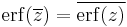
$\operatorname{erf} (\overline{z}) = \overline{\operatorname{erf}(z)}$

where $\overline{z}$ is the complex conjugate of z.

The integrand ƒ = exp(−z²) and ƒ = erf(z) are shown in the complex z-plane in figures 2 and 3. Level of Im(ƒ) = 0 is shown with a thick green line. Negative integer values of Im(ƒ) are shown with thick red lines. Positive integer values of $\Im(f)$ are shown with thick blue lines. Intermediate levels of Im(ƒ) = constant are shown with thin green lines. Intermediate levels of Re(ƒ) = constant are shown with thin red lines for negative values and with thin blue lines for positive values.

At the real axis, erf(z) approaches unity at z → +∞ and −1 at z → −∞. At the imaginary axis, it tends to ±i∞.

Taylor series

The error function is an entire function; it has no singularities (except that at infinity) and its Taylor expansion always converges.

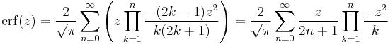
The defining integral cannot be evaluated in closed form in terms of elementary functions, but by expanding the integrand e^−z² into its Taylor series and integrating term by term, one obtains the error function's Taylor series as:

$\operatorname{erf}(z)= \frac{2}{\sqrt{\pi}}\sum_{n=0}^\infin\frac{(-1)^n z^{2n%2B1}}{n! (2n%2B1)} =\frac{2}{\sqrt{\pi}} \left(z-\frac{z^3}{3}%2B\frac{z^5}{10}-\frac{z^7}{42}%2B\frac{z^9}{216}-\ \cdots\right)$

which holds for every complex number z. The denominator terms are sequence A007680 in the OEIS.

For iterative calculation of the above series, the following alternative formulation may be useful:

$\operatorname{erf}(z)= \frac{2}{\sqrt{\pi}}\sum_{n=0}^\infin\left(z \prod_{k=1}^n {\frac{-(2k-1) z^2}{k (2k%2B1)}}\right) = \frac{2}{\sqrt{\pi}} \sum_{n=0}^\infin \frac{z}{2n%2B1} \prod_{k=1}^n \frac{-z^2}{k}$

because $\frac{-(2k-1) z^2}{k (2k%2B1)}$ expresses the multiplier to turn the k^th term into the (k + 1)^th term (considering z as the first term).

The error function at +∞ is exactly 1 (see Gaussian integral).

The derivative of the error function follows immediately from its definition:

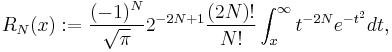
$\frac{\rm d}{{\rm d}z}\,\mathrm{erf}(z)=\frac{2}{\sqrt{\pi}}\,e^{-z^2}.$

An antiderivative of the error function is

$z\,\operatorname{erf}(z) %2B \frac{e^{-z^2}}{\sqrt{\pi}}.$

Inverse functions

The inverse error function can be defined in terms of the Maclaurin series

$\operatorname{erf}^{-1}(z)=\sum_{k=0}^\infin\frac{c_k}{2k%2B1}\left (\frac{\sqrt{\pi}}{2}z\right )^{2k%2B1}, \,\!$

where c₀ = 1 and

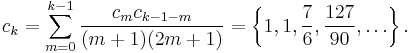
$c_k=\sum_{m=0}^{k-1}\frac{c_m c_{k-1-m}}{(m%2B1)(2m%2B1)} = \left\{1,1,\frac{7}{6},\frac{127}{90},\ldots\right\}.$

So we have the series expansion (note that common factors have been canceled from numerators and denominators):

$\operatorname{erf}^{-1}(z)=\tfrac{1}{2}\sqrt{\pi}\left (z%2B\frac{\pi}{12}z^3%2B\frac{7\pi^2}{480}z^5%2B\frac{127\pi^3}{40320}z^7%2B\frac{4369\pi^4}{5806080}z^9%2B\frac{34807\pi^5}{182476800}z^{11}%2B\cdots\right ).\$

(After cancellation the numerator/denominator fractions are entries A092676/A132467 in the OEIS; without cancellation the numerator terms are given in entry A002067.) Note that the error function's value at ±∞ is equal to ±1.

The inverse complementary error function is defined as

$\operatorname{erfc}^{-1}(1-z) = \operatorname{erf}^{-1}(z).$

Asymptotic expansion

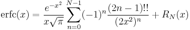
A useful asymptotic expansion of the complementary error function (and therefore also of the error function) for large x is

$\mathrm{erfc}(x) = \frac{e^{-x^2}}{x\sqrt{\pi}}\left [1%2B\sum_{n=1}^\infty (-1)^n \frac{1\cdot3\cdot5\cdots(2n-1)}{(2x^2)^n}\right ]=\frac{e^{-x^2}}{x\sqrt{\pi}}\sum_{n=0}^\infty (-1)^n \frac{(2n-1)!!}{(2x^2)^n}.\,$

This series diverges for every finite x, and its meaning as asymptotic expansion is that, for any $N\in\N$ one has

$\mathrm{erfc}(x) = \frac{e^{-x^2}}{x\sqrt{\pi}}\sum_{n=0}^{N-1} (-1)^n \frac{(2n-1)!!}{(2x^2)^n}%2B R_N(x) \,$

where the remainder, in Landau notation, is

$R_N(x)=O(x^{-2N%2B1} e^{-x^2})$ as $x\to\infty$ .

Indeed, the exact value of the remainder is

$R_N(x):= \frac{(-1)^N}{\sqrt{\pi}}2^{-2N%2B1}\frac{(2N)!}{N!}\int_x^\infty t^{-2N}e^{-t^2} dt,$

which follows easily by induction, writing 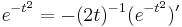$e^{-t^2}=-(2t)^{-1}(e^{-t^2})'$ and integrating by parts.

For large enough values of x, only the first few terms of this asymptotic expansion are needed to obtain a good approximation of erfc(x) (while for not too large values of x note that the above Taylor expansion at 0 provides a very fast convergence).

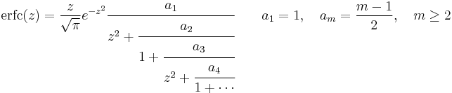
Continued fractions expansion

A continued fractions expansion of the complementary error function is ^[1]:

$\mathrm{erfc}(z) = \frac{z}{\sqrt{\pi}}e^{-z^2} \cfrac{a_1}{z^2%2B \cfrac{a_2}{1%2B \cfrac{a_3}{z^2%2B \cfrac{a_4}{1%2B\dotsb}}}} \qquad a_1 = 1,\quad a_m = \frac{m-1}{2},\quad m \geq 2$

Approximation with elementary functions

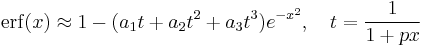
Abramowitz and Stegun give several approximations of varying accuracy (equations 7.1.25-28). This allows one to choose the fastest approximation suitable for a given application. In order of increasing accuracy, they are:

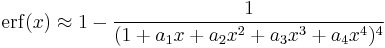$\operatorname{erf}(x)\approx 1-\frac{1}{(1%2Ba_1x%2Ba_2x^2%2Ba_3x^3%2Ba_4x^4)^4}$ (maximum error: 5·10^-4)

where a₁=0.278393, a₂=0.230389, a₃=0.000972, a₄=0.078108

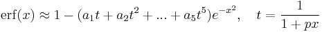
$\operatorname{erf}(x)\approx 1-(a_1t%2Ba_2t^2%2Ba_3t^3)e^{-x^2},\quad t=\frac{1}{1%2Bpx}$ (maximum error: 2.5·10^-5)

where p=0.47047, a₁=0.3480242, a₂=-0.0958798, a₃=0.7478556

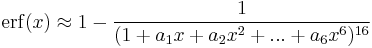$\operatorname{erf}(x)\approx 1-\frac{1}{(1%2Ba_1x%2Ba_2x^2%2B...%2Ba_6x^6)^{16}}$ (maximum error: 3·10^-7)

where a₁=0.0705230784, a₂=0.0422820123, a₃=0.0092705272, a₄=0.0001520143, a₅=0.0002765672, a₆=0.0000430638

$\operatorname{erf}(x)\approx 1-(a_1t%2Ba_2t^2%2B...%2Ba_5t^5)e^{-x^2},\quad t=\frac{1}{1%2Bpx}$ (maximum error: 1.5·10^-7)

where p=0.3275911, a₁=0.254829592, a₂=-0.284496736, a₃=1.421413741, a₄=-1.453152027, a₅=1.061405429

All of these approximations are valid for x≥0. To use these approximations for negative x, use the fact that erf(x) is an odd function, so erf(x)=-erf(-x).

Another approximation is given by

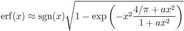
$\operatorname{erf}(x)\approx \sgn(x) \sqrt{1-\exp\left(-x^2\frac{4/\pi%2Bax^2}{1%2Bax^2}\right)}$

where

$a = \frac{8(\pi-3)}{3\pi(4-\pi)} \approx 0.140012.$

This is designed to be very accurate in a neighborhood of 0 and a neighborhood of infinity, and the error is less than 0.00035 for all x. Using the alternate value a ≈ 0.147 reduces the maximum error to about 0.00012.^[2]

This approximation can also be inverted to calculate the inverse error function:

$\operatorname{erf}^{-1}(x)\approx \sgn(x) \sqrt{\sqrt{\left(\frac{2}{\pi a}%2B\frac{\ln(1-x^2)}{2}\right)^2 - \frac{\ln(1-x^2)}{a}} -\left(\frac{2}{\pi a}%2B\frac{\ln(1-x^2)}{2}\right)}$

Applications

When the results of a series of measurements are described by a normal distribution with standard deviation $\scriptstyle\sigma$ and expected value 0, then $\scriptstyle\operatorname{erf}\,\left(\,\frac{a}{\sigma \sqrt{2}}\,\right)$ is the probability that the error of a single measurement lies between −a and +a, for positive a. This is useful, for example, in determining the bit error rate of a digital communication system.

The error and complementary error functions occur, for example, in solutions of the heat equation when boundary conditions are given by the Heaviside step function.

Related functions

The error function is essentially identical to the standard normal cumulative distribution function, denoted Φ, also named norm(x) by software languages, as they differ only by scaling and translation. Indeed,

$\Phi(x) =\tfrac{1}{\sqrt{2\pi}}\int_{-\infty}^x e^\tfrac{-t^2}{2} dt = \tfrac{1}{2}\left[1%2B\mbox{erf}\left(\frac{x}{\sqrt{2}}\right)\right]=\tfrac{1}{2}\,\mbox{erfc}\left(-\frac{x}{\sqrt{2}}\right)$

or rearranged for erf and erfc:

$\begin{align} \mathrm{erf}(x) &= 2 \Phi \left ( x \sqrt{2} \right ) - 1 \\ \mathrm{erfc}(x) &= 2 \Phi \left ( - x \sqrt{2} \right ). \end{align}$

Consequently, the error function is also closely related to the Q-function, which is the tail probability of the standard normal distribution. The Q-function can be expressed in terms of the error function as

$Q(x) =\tfrac{1}{2} - \tfrac{1}{2} \operatorname{erf} \Bigl( \frac{x}{\sqrt{2}} \Bigr)=\tfrac{1}{2}\operatorname{erfc}(\frac{x}{\sqrt{2}}).$

The inverse of $\scriptstyle\Phi\,$ is known as the normal quantile function, or probit function and may be expressed in terms of the inverse error function as

$\operatorname{probit}(p) = \Phi^{-1}(p) = \sqrt{2}\,\operatorname{erf}^{-1}(2p-1) = -\sqrt{2}\,\operatorname{erfc}^{-1}(2p).$

The standard normal cdf is used more often in probability and statistics, and the error function is used more often in other branches of mathematics.

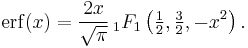
The error function is a special case of the Mittag-Leffler function, and can also be expressed as a confluent hypergeometric function (Kummer's function):

$\mathrm{erf}(x)= \frac{2x}{\sqrt{\pi}}\,_1F_1\left(\tfrac12,\tfrac32,-x^2\right).$

It has a simple expression in terms of the Fresnel integral. In terms of the Regularized Gamma function P and the incomplete gamma function,

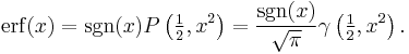
$\operatorname{erf}(x)=\operatorname{sgn}(x) P\left(\tfrac12, x^2\right)={\operatorname{sgn}(x) \over \sqrt{\pi}}\gamma\left(\tfrac12, x^2\right).$

$\scriptstyle\operatorname{sgn}(x) \$ is the sign function.

Generalized error functions

Some authors discuss the more general functions:

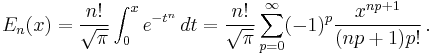
$E_n(x) = \frac{n!}{\sqrt{\pi}} \int_0^x e^{-t^n}\,dt =\frac{n!}{\sqrt{\pi}}\sum_{p=0}^\infin(-1)^p\frac{x^{np%2B1}}{(np%2B1)p!}\,.$

Notable cases are:

E₀(x) is a straight line through the origin: $\scriptstyle E_0(x)=\frac{x}{e \sqrt{\pi}}$
E₂(x) is the error function, erf(x).

After division by n!, all the E_n for odd n look similar (but not identical) to each other. Similarly, the E_n for even n look similar (but not identical) to each other after a simple division by n!. All generalised error functions for n > 0 look similar on the positive x side of the graph.

These generalised functions can equivalently be expressed for x > 0 using the Gamma function and incomplete Gamma function:

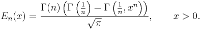
$E_n(x) = \frac{\Gamma(n)\left(\Gamma\left(\frac{1}{n}\right)-\Gamma\left(\frac{1}{n},x^n\right)\right)}{\sqrt\pi}, \quad \quad x>0.\$

Therefore, we can define the error function in terms of the incomplete Gamma function:

$\operatorname{erf}(x) = 1 - \frac{\Gamma\left(\frac{1}{2},x^2\right)}{\sqrt\pi}.\$

Iterated integrals of the complementary error function

The iterated integrals of the complementary error function are defined by

$\mathrm i^n \operatorname{erfc}\, (z) = \int_z^\infty \mathrm i^{n-1} \operatorname{erfc}\, (\zeta)\;\mathrm d \zeta.\,$

They have the power series

$\mathrm i^n \operatorname{erfc}\, (z) = \sum_{j=0}^\infty \frac{(-z)^j}{2^{n-j}j! \Gamma \left( 1 %2B \frac{n-j}{2}\right)}\,,$

from which follow the symmetry properties

$\mathrm i^{2m} \operatorname{erfc} (-z) = - \mathrm i^{2m} \operatorname{erfc}\, (z) %2B \sum_{q=0}^m \frac{z^{2q}}{2^{2(m-q)-1}(2q)! (m-q)!}$

and

$\mathrm i^{2m%2B1} \operatorname{erfc} (-z) = \mathrm i^{2m%2B1} \operatorname{erfc}\, (z) %2B \sum_{q=0}^m \frac{z^{2q%2B1}}{2^{2(m-q)-1}(2q%2B1)! (m-q)!}\,.$

Implementations

C: C99 provides the functions double erf(double x) and double erfc(double x) in the header math.h. The pairs of functions {erff(),erfcf()} and {erfl(),erfcl()} take and return values of type float and long double respectively.

C++: C++11 provides erf() and erfc() in the header cmath. Both functions are overloaded to accept arguments of type float, double, and long double.

Fortran: The Fortran 2008 standard provides the ERF, ERFC and ERFC_SCALED functions to calculate the error function and its complement.

Python: Included since version 2.7 as math.erf(). For previous version, an implementation of erf for complex arguments is in SciPy as scipy.special.erf()^[3] and also in the arbitrary-precision arithmetic mpmath library as mpmath.erf()

Mathematica: erf is implemented as Erf and Erfc in Mathematica

Haskell (programming language): An erf package^[4] exists that provides a typeclass for the error function and implementations for the native floating point types

R: "The so-called 'error function'"^[5] is not provided directly, but is detailed as an example of the normal cumulative distribution function (?pnorm), which is based on W. J. Cody's rational Chebyshev approximation algorithm.^[6]

Matlab provides both erf and erfc, also via W. J. Cody's algorithm.

Ruby: Provides Math.erf() and Math.erfc().

Table of values

x	erf(x)	erfc(x)	x	erf(x)	erfc(x)
0.00	0.0000000	1.0000000	1.30	0.9340079	0.0659921
0.05	0.0563720	0.9436280	1.40	0.9522851	0.0477149
0.10	0.1124629	0.8875371	1.50	0.9661051	0.0338949
0.15	0.1679960	0.8320040	1.60	0.9763484	0.0236516
0.20	0.2227026	0.7772974	1.70	0.9837905	0.0162095
0.25	0.2763264	0.7236736	1.80	0.9890905	0.0109095
0.30	0.3286268	0.6713732	1.90	0.9927904	0.0072096
0.35	0.3793821	0.6206179	2.00	0.9953223	0.0046777
0.40	0.4283924	0.5716076	2.10	0.9970205	0.0029795
0.45	0.4754817	0.5245183	2.20	0.9981372	0.0018628
0.50	0.5204999	0.4795001	2.30	0.9988568	0.0011432
0.55	0.5633234	0.4366766	2.40	0.9993115	0.0006885
0.60	0.6038561	0.3961439	2.50	0.9995930	0.0004070
0.65	0.6420293	0.3579707	2.60	0.9997640	0.0002360
0.70	0.6778012	0.3221988	2.70	0.9998657	0.0001343
0.75	0.7111556	0.2888444	2.80	0.9999250	0.0000750
0.80	0.7421010	0.2578990	2.90	0.9999589	0.0000411
0.85	0.7706681	0.2293319	3.00	0.9999779	0.0000221
0.90	0.7969082	0.2030918	3.10	0.9999884	0.0000116
0.95	0.8208908	0.1791092	3.20	0.9999940	0.0000060
1.00	0.8427008	0.1572992	3.30	0.9999969	0.0000031
1.10	0.8802051	0.1197949	3.40	0.9999985	0.0000015
1.20	0.9103140	0.0896860	3.50	0.9999993	0.0000007

x	erfc(x)/2
1	0.0786496
2	0.00233887
3	1.10452e-05
4	7.70863e-09
5	7.6873e-13
6	1.07599e-17
7	2.09191e-23
8	5.61215e-30
9	2.06852e-37
10	1.04424e-45
11	7.20433e-55
12	6.78131e-65
13	8.69779e-76
14	1.51861e-87
15	3.6065e-100
16	1.16424e-113
17	5.10614e-128
18	3.04118e-143
19	2.45886e-159
20	2.69793e-176
21	4.01623e-194
22	8.10953e-213
23	2.22063e-232
24	8.24491e-253
25	4.15009e-274
26	2.8316e-296
27	2.61855e-319

References

^ Cuyt, A.A.M.; Petersen, V.; Verdonk, B.; Waadeland, H.; Jones, W.B. (2008). Handbook of Continued Fractions for Special Functions. Springer-Verlag. ISBN 978-1-4020-6948-2.
^ Winitzki, Sergei (6 February 2008). "A handy approximation for the error function and its inverse" (PDF). http://sites.google.com/site/winitzki/sergei-winitzkis-files/erf-approx.pdf. Retrieved 2011-10-03.
^ http://docs.scipy.org/doc/scipy/reference/generated/scipy.special.erf.html
^ http://hackage.haskell.org/package/erf
^ R Development Core Team (2011-02-25), R: The Normal Distribution, http://stat.ethz.ch/R-manual/R-patched/library/stats/html/Normal.html
^ Cody, W. J. (1969). "Rational Chebyshev Approximations for the Error Function". Math. Comp. 23 (107): 631–637. http://www.ams.org/journals/mcom/1969-23-107/S0025-5718-1969-0247736-4/S0025-5718-1969-0247736-4.pdf.

Abramowitz, Milton; Stegun, Irene A., eds. (1965), "Chapter 7", Handbook of Mathematical Functions with Formulas, Graphs, and Mathematical Tables, New York: Dover, pp. 297, ISBN 978-0486612720, MR 0167642, http://www.math.sfu.ca/~cbm/aands/page_297.htm .
Press, WH; Teukolsky, SA; Vetterling, WT; Flannery, BP (2007), "Section 6.2. Incomplete Gamma Function and Error Function", Numerical Recipes: The Art of Scientific Computing (3rd ed.), New York: Cambridge University Press, ISBN 978-0-521-88068-8, http://apps.nrbook.com/empanel/index.html#pg=259

Temme, N. M. (2010), "Error Functions, Dawson’s and Fresnel Integrals", in Olver, Frank W. J.; Lozier, Daniel M.; Boisvert, Ronald F. et al., NIST Handbook of Mathematical Functions, Cambridge University Press, ISBN 978-0521192255, MR 2723248, http://dlmf.nist.gov/7

External links

MathWorld – Erf

/sub>=-1.453152027, a

Error function

Contents

The name "error function"

Properties

Taylor series

Inverse functions

Asymptotic expansion

Continued fractions expansion

Approximation with elementary functions

Applications

Related functions

Generalized error functions

Iterated integrals of the complementary error function

Implementations

Table of values

See also

Related functions

In probability

References

External links